Load TikZ in either one way.
\documentclass[tikz, border=2pt]{standalone}\usepackage{tikz}
Graph
With pgfplots
PGF Plots automizes the axes configurations, for example:
- major and minor ticks and labels on the axes
- major and minor grid lines
- legend styles and positioning
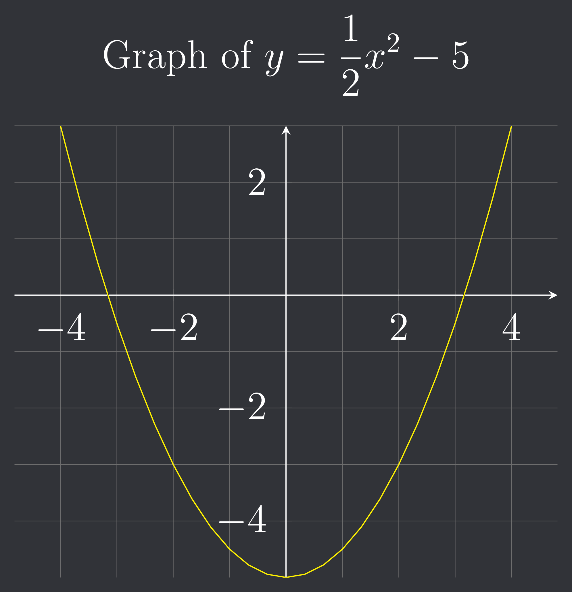
Simplest example for Discord:
\begin{tikzpicture}[declare function={f(\x)=(\x)^2/2 - 5;}]
\begin{axis}[
  axis equal,
  grid=both,
  grid style={line width=.2pt, draw=gray},
  minor tick num=1,
  xtick={-4,-2,...,4},
  ytick={-4,-2,...,4},
  axis lines=center,
  title={Graph of $y = \frac12 x^2 - 5$},
]
\addplot[yellow,domain=-4:4] {f(\x)};
\pgfplotsset{
  grid style={gray},
  major grid style={gray,line width=0.7}
}
\end{axis}
\end{tikzpicture}
TeXit’s output:
Explanation for the code:
\usepackage{pgfplots}: load package\pgfplotsset{compat=1.18}: set dependency\pgfplotsset{grid style={gray}}: draw grid lines\pgfplotsset{major grid style={gray,line width=1}}: thicker major grid linesaxis equal: x and y-distances are in 1:1 ratioaxis lines=center: axes passes through the origingrid=both: enable major grid linesminor tick num=9: draw 9 minor grid lines between each pair of major grid linesxlabel={$x$},ylabel={$y$}: labels for the axestitle={}: title of a graphlegend style={at={(0,-0.05)},anchor=north west,fill=none}: legend stylesat={(0,-0.05)}coordinates relative to the entire PGF plot.(0,0)and(1,1)represent the bottom left and top right corners respectively.anchor=north west: relative to the top left corner of the entire legend boxfill=none: (for TeXit) transparent background. TeXit renders a black background by default.
\begin{scope}[thick, samples=201, smooth]: avoid repetition of codeblue!20is a shorthand forblue!20!white, meaning 20% blue and 80% white.
\documentclass[tikz,border=2pt]{standalone}
\usepackage{pgfplots}
\pgfplotsset{compat=1.18}
\begin{document}
\pgfplotsset{
    grid style={gray},
    major grid style={gray,line width=0.7}
}
\begin{tikzpicture}
\begin{axis}[
    axis equal,
    axis lines=center,
    grid=both,
    minor tick num=9,
    xlabel={$x$},
    ylabel={$y$},
    title={Another \LaTeX{} graph},
    legend style={at={(0,-0.05)},anchor=north west,fill=none}
    ]
    \begin{scope}[thick, samples=201, smooth]
    \addplot[domain=-2.3:2.3, yellow] (x,{0.5 * x^2 - 1.5 * x - 4});
    \addlegendentry{$y = 0.5x^2-1.5x-4$};
    \addplot[domain=0:360,variable=\t, blue!20] ({sqrt(5) * cos(t)}, {sqrt(5) * sin(t)});
    \addlegendentry{$x^2+y^2=5$};
    \end{scope}
\end{axis}
\end{tikzpicture}
\end{document}

\pgfplotsset{
    grid style={gray,opacity=0.3},
    major grid style={gray,line width=1,opacity=0.3}
}
\begin{tikzpicture}
\begin{axis}[
    axis equal,
    axis lines=center,
    grid=both,
    xmin=-9,
    xmax=3,
    ymin=-5,
    ymax=7,
    minor tick num=9,
    xlabel={$\mathrm{Re}(z)$},
    ylabel={$\mathrm{Im}(z)$},
    title={Sample \LaTeX{} complex plot},
    enlargelimits={abs=0.5},
    disabledatascaling,
]
\draw[red!40,fill=red!40,fill opacity=0.3] (-5,0) circle [radius=4];
\node at (-6.8,2.2) [red!30,rotate=45]{\scriptsize $|z+5| \le 4$};
\begin{scope}
    \clip (current axis.south west) rectangle (current axis.north east);
    \draw[fill=yellow,fill opacity=0.3] (-15,-10) -- (5,10) -- (current axis.south east) -- cycle;
    \node at (current axis.south east) [anchor=south east, yellow]{\scriptsize $\mathrm{Re}(ze^{i \pi/4}) \ge -5/\sqrt{2}$};
\end{scope}
\end{axis}
\end{tikzpicture}

Special technical features of the above graph:
axis equal: ensure that the circle isn’t shown as an ellipse.disabledatascaling: ensure that the circle is shown.- grid lines: I found that
opacity=0.3withline width=1suitsgray. - graph limits: I first tried
xmin=-9andxmax=3, but withoutymin=-5andymax=7, I only got the graph of about [-1.5,1.5] × [-1,2]. enlargelimits={abs=0.5}: to ensure that the tips of the axes don’t overlap the labels forxmaxandymax.- the default
cs(coordinate system) isaxis csinside theaxisenvironment. This allows a simple syntax for a TikZ circle with[radius=<r>]. node at (P) [rotate=<deg>]{text}: rotate node content by<deg>anticlockwise.fill opacity=0.3: shade the region with a light color, so that the math expression of the region can be written inside the filling.current axis: contains points related to the two ends of each axis.
Code sample for a sample data plot
\documentclass[tikz,border=2pt]{standalone}
\usepackage{pgfplots}
\pgfplotsset{compat=1.18}
\begin{document}
\begin{tikzpicture}
\begin{axis} [
title={sample \LaTeX{} graph},
axis lines=middle,
xlabel near ticks,
ylabel near ticks,
xlabel={$t$ time (s)},
ylabel={$h$ distance (cm)},
xmin=0,
xmax=0.5,
ymin=0,
ymax=80,
xtick={0,0.1,...,0.5},
ytick={0,20,...,80},
grid=both,
minor tick num=9,
grid style={line width=.1pt, draw=black!50},
major grid style={line width=.5pt,draw=black!50},
legend style={at={(1.05,1)},anchor=north west,fill=none},
enlargelimits=0.05,
]
\addplot[mark=*,thick] coordinates {
(0,0)
(0.1,20)
(0.2,40)
(0.3,60)
(0.4,80)
};
\addlegendentry{line 1}
\addplot[mark=*,thick,blue!50] coordinates {
(0.05,3.4)
(0.16,21.7)
(0.24,37.6)
(0.33,64.4)
(0.49,78.2)
};
\addlegendentry{line 2}
\end{axis}
\end{tikzpicture}
\end{document}

The $\LaTeX$ in the graph’s title has to be replaced by \LaTeX{} to avoid
the error message
You can't use `\spacefactor' in math mode.
A large part of the code is copied from TeX.SE exchange.
\pgfplotsset{
    grid style={gray},
    major grid style={gray,line width=1},
    trig format plots=rad,
    legend columns=2,
}
\pgfmathsetmacro{\PI}{3.141592654}
\begin{tikzpicture}
\begin{axis}[axis lines=center,grid=both,
    xmin=-0.5*\PI,
    xmax=2.5*\PI,
    ymin=-1.5,
    ymax=1.5,
    restrict y to domain=-1.5:1.5,
    minor tick num=9,
    xlabel={$x$},
    ylabel={$y$},
    scaled x ticks={real:\PI},
    xtick scale label code/.code={},
    xtick distance=\PI/2,
    xticklabel={
        \ifdim \tick pt = 1 pt
            \strut$\pi$
        \else\ifdim \tick pt = -1 pt
            \strut$-\pi$
        \else
            \pgfmathparse{round(10*\tick)/10}
            \pgfmathifisint{\pgfmathresult}{%
                \strut$\pgfmathprintnumber[int detect]{\pgfmathresult}\pi$
            }{%
                \strut$\pgfmathprintnumber{\pgfmathresult}\pi$
            }
        \fi\fi
    },
    xticklabel style={
        /pgf/number format/frac,
        /pgf/number format/frac whole=false,
    },
    title={Sample \LaTeX{} trigonometric graph},
    legend style={at={(0,-0.05)},anchor=north west,fill=none},
    enlargelimits={abs=0.2},
]
\begin{scope}[thick,domain=-pi/2:2.5*pi,samples=201,smooth,mark=none]
\addplot+ {sin(x)};
\addlegendentry{$y=\sin(x)$};
\addplot+ {cos(x)};
\addlegendentry{$y = \cos(x)$};
\addplot+[dashed] {tan(x)};
\addlegendentry{$y = \tan(x)$};
\end{scope}
\foreach \k in {0,0.5,...,2} {\addplot[dashed] coordinates{({\k * \PI},-1.5) ({\k * \PI},1.5)};}
\end{axis}
\end{tikzpicture}
\pgfmathsetmacro{\PI}{3.141592654}: without this, the calculated\tickwould become a strange fraction rather than π/2 whenxtick distance=\PI.scaled x ticks={real: \PI}: tick number\tickis divided by\PI. Outsidexticklabel, the x-coordinate can be used as usual.xticklabelandxticklabel style: set number plotting to fractions. In case that the numbers are ±1, the\ifdimwould isolate the case, and omit the ‘1’ in the result.restrict y to domain=-1.5:1.5: avoid tangent curves from bumping up the frame.

Without pgfplot
An example copied from Discord.
\begin{tikzpicture}
    \draw[help lines,step=1 cm](-4.9,-3.9) grid (4.9,3.9);

    % shaded region
    \fill [gray, domain=-2:2, variable=\x]
    (-2, 0)
    -- plot ({\x}, {\x-1})
    -- (2, 0)
    -- cycle;

    % x-axis
    \draw [thick] [->] (-5,0)--(5,0) node[right, below] {$x$};
    \foreach \x in {-4,...,4}
    \draw[xshift=\x cm, thick] (0pt,-1pt)--(0pt,1pt) node[below] {$\x$};

    % y-axis
    \draw [thick] [->] (0,-4)--(0,4) node[above, left] {$y$};
    \foreach \y in {-3,...,3}
    \draw[yshift=\y cm, thick] (-1pt,0pt)--(1pt,0pt) node[left] {$\y$};

    % function plot(s)
    \draw [domain=-2:2, variable=\x]
    plot ({\x}, {\x*\x}) node[right] at (1.5,2) {$f(x)=x^2$};

    \draw [domain=-2:3.5, variable=\x] plot ({\x}, {\x-1});
\end{tikzpicture}

Geometry
2D
\begin{tikzpicture}
\draw[<->, >=latex, thick] (-3,0) -- (3,0) node [below, pos=0.5] {6 cm};
\draw[thick] circle (3);
\draw (0,0) node {$\bullet$};
\end{tikzpicture}

\begin{tikzpicture}[scale=0.5]
  \draw (0,0) rectangle (3,7);
\end{tikzpicture}

Right-angled triangle with the right angle mark.
\begin{tikzpicture}[scale=0.5]
\coordinate (O) at (0,0);
\coordinate (B) at (12,0);
\coordinate (H) at (0,16);
\draw[thick] (O) node [below left] {$O$}
-- (B) node [below, pos=0.5]{12} node [right] {$B$}
-- (H) node [above] {$H$}
-- cycle node [left, pos=0.5] {16};
\draw[thick] (0,1) -- (1,1) -- (1,0);
\end{tikzpicture}

Angle with mark.
\draw (x,y) arc (start:stop:radius); draws an arc.
\begin{tikzpicture}[scale=0.5]
\draw (0,0) node[below] {$O$};
\draw (2,0) node[right] {$A$};
\draw (2,2) node[right] {$B$};
\draw (0,0) -- (2,0);
\draw (0,0) -- (2,2);
\draw (1,0) arc (0:45:1);
\end{tikzpicture}

\newcommand\myvar{value}before\begin{document}radius: radius length (i.e. distance of a vertex to the center),\ris used by the system.n: number of sidesdTheta: size of angle of a sector\the\numexpr\n-1: evaluten − 1.- I’m not sure if
\n - 1triggers an error because\nmight be interpreted as text. \numexpr\n-1means\n-1is a numerical expression.\thepreceeding\numexprevaluates this expression.
- I’m not sure if
\foreach \x in {1,...,m} {[cmd in terms of \x]}: use for loop to avoid repetition.
Improved stand alone example of regular polygon.
\newcommand\myR{2}
\newcommand\n{7}
\newcommand\dTheta{360/\n}
\tikzset{
  every node/.style={draw,fill,circle,minimum size=6pt,inner sep=-2pt,},
  label distance=2.5mm,
}
\begin{tikzpicture}
  \foreach \k in {1,...,\n} {
    \node[label=\k*\dTheta:$V_{\k}$] (V\k) at ({\dTheta*\k}:\myR){};
  }
  \draw (V1.center) foreach \k in {2,...,\n} { -- (V\k.center)} -- cycle;
\end{tikzpicture}
every node/.styleapplies a series of styles inside[...]to every node.node {$\bullet$}can’t represent the actual position described by the character ‘•’.minimum sizeis the minimum diameter of the circular dot.inner sepis the “signed space” between the perimeter of the content box and the node’s boundary (rendered bydraw).
- I’ve tried
\draw (V1) -- foreach ... {} -- cyclebut I got a logic error: the node edges were connected to the node boundary instead of the coordinate(V\k.center). This is known as TikZ’s “path shortening” effect, which is deactivated . - I’ve used an empty
\nodewith alabel=<angle>:<text>instead of a\coordinatewith apin=<angle>:<text>because\coordinateis a shorthand of\node[shape=coordinate], but I’m using a circular dot\node[draw,fill,shape=circle]to mark the actual position of the vertex. As a result, the actualshape=circle.- I don’t want any pin edges. It would be more sensible to use
labels instead ofpins withevery pin edge/.style={opacity=0}.

3D
\usetikzlibrary{3d} in the preamble.
Simplest example to how coordinates are presented.
\begin{tikzpicture}
  \draw[-latex] (0,0,0)--(1,0,0) node[pos=1.5]{$\vec{i}$};
  \draw[-latex] (0,0,0)--(0,1,0) node[pos=1.5]{$\vec{j}$};
  \draw[-latex] (0,0,0)--(0,0,1) node[pos=1.5]{$\vec{k}$};
  \foreach \k in {0,1} {\draw (0,0,\k)--(1,0,\k)--(1,1,\k)--(0,1,\k)--cycle;}
  \foreach \i in {0,1} \foreach \j in {0,1} \draw (\i,\j,0)--(\i,\j,1);
\end{tikzpicture}

You might want the z-axis pointing upwards and the y-axis pointing to the
right. TikZ pour l’impatient has provided a handy math3d style for that.
\documentclass[preview,tikz]{standalone}
\usetikzlibrary{3d}
\begin{document}
\begin{tikzpicture}
[
  math3d/.style={x= {(-0.353cm,-0.353cm)},z={(0cm,1cm)},y={(1cm,0cm)}},
]
\draw[-latex,math3d] (0,0,0)--(1,0,0) node[pos=1.5]{$\vec{i}$};
\draw[-latex,math3d] (0,0,0)--(0,1,0) node[pos=1.5]{$\vec{j}$};
\draw[-latex,math3d] (0,0,0)--(0,0,1) node[pos=1.5]{$\vec{k}$};
\foreach \k in {0,1} {\draw (0,0,\k)--(1,0,\k)--(1,1,\k)--(0,1,\k)--cycle;}
\foreach \i in {0,1} \foreach \j in {0,1} \draw (\i,\j,0)--(\i,\j,1);
\end{tikzpicture}
\end{document}

\documentclass[preview,tikz]{standalone}
\usetikzlibrary{3d}
\begin{document}
\begin{tikzpicture}
[
  every node/.style={draw,fill,circle,minimum size=6pt,inner sep=-2pt,},
  x= {(-0.353cm,-0.353cm)}, z={(0cm,1cm)},y={(1cm,0cm)},
]
\pgfmathsetmacro\myR{2}
\pgfmathsetmacro\n{7}
\pgfmathsetmacro\dTheta{360/\n}
\pgfmathsetmacro\myH{3}
\foreach \lvl in {0,\myH} {
  \foreach \k in {1,...,\n} {
    \node (L\lvl V\k) at (xyz cylindrical cs:radius=\myR, angle={\dTheta * \k}, z=\lvl) {};
  }
}
\foreach \lvl in {0,\myH} {
  \draw[dashed] (L\lvl V1.center) foreach \k in {2,...,\n} { -- (L\lvl V\k.center)} -- cycle;
}
\foreach \k in {1,...,\n} {
  \draw[dashed] (L0V\k.center) -- (L\myH V\k.center);
}
\end{tikzpicture}
\end{document}
The space between L0 and V\k.center is taken away to avoid compilation
error.

\documentclass[preview,tikz]{standalone}
\usetikzlibrary{3d}
\begin{document}
\begin{tikzpicture}
[
  every node/.style={draw,fill,circle,minimum size=6pt,inner sep=-2pt,},
  x= {(-0.353cm,-0.353cm)}, z={(0cm,1cm)},y={(1cm,0cm)},
]
\pgfmathsetmacro\myR{2}
\pgfmathsetmacro\n{7}
\pgfmathsetmacro\dTheta{360/\n}
\pgfmathsetmacro\myH{3}
\node (apex) at (0,0,\myH) {};
\foreach \k in {1,...,\n} {
  \node (V\k) at (xyz cylindrical cs:radius=\myR, angle={\dTheta * \k}, z=0) {};
}
\draw[dashed] (V1.center) foreach \k in {2,...,\n} { -- (V\k.center)} -- cycle;
\foreach \k in {1,...,\n} {\draw[dashed] (apex) -- (V\k.center);}
\end{tikzpicture}
\end{document}

Generate from Geogebra
99% of the guide/docs use Desktop version. Luckily, this Geogebra help thread provides a way to convert Geogebra figures to TikZ code on the web app.
const patNum = /[\d]+(\.([\d]+))?/g
const rplNum = a => Math.round((parseFloat(a)+Number.EPSILON)*100)/100
const patColor=/\\definecolor{(?<color>[a-z]+)}/g
const patLw=/line width=(\d+\.?\d*)pt/g
const rplLw = a => `lw${a.replace('.','p')}`
const axes = ['x', 'y']
const bddtypes = ['min', 'max']
const PGF_VERSION = 1.18
let myApp
let appNum = 0
new Function(`myApp = ${$('[id^="ggbApplet"]')[appNum].id}`)()
myApp.exportPGF(function(a){
  const SCALE_FACTOR = rplNum(50/Math.max(...a.match(patNum).map(a=>parseFloat(a))))
  // build the array of colors
  let myColors = []
  while((match = patColor.exec(a)) !== null) {
    let color = match.groups.color
    for (var i = 1; i <= color.length; i++) {
      let colorShort = color.substring(0,i)
      if (myColors.find(c=>c.colorShort==colorShort) == null) {
        myColors.push({color:color,colorShort:colorShort})
        break
      }
    }
  }
  // round to 2dp, remove unnecessary styles, inject custom style holder
  let output = a.replace(patNum,rplNum)
    .replace(/\[10pt\]{article}/,'{standalone}')
    .replace(/(compat=)\d+\.\d+/,`$1${PGF_VERSION}`)
    .replace(/^\\usepackage{mathrsfs}\s*\\usetikzlibrary{arrows}\s*\\pagestyle{empty}\s*\n/m,'')
    .replace(/(\\begin{tikzpicture}\[)(.*)(\])/,`$1scale=${SCALE_FACTOR}$3`)
    .replace(/(?=\\begin{tikzpicture})/,'\\tikzset{\n}\n')
  // replace color=, fill= with short names
  const myIdx = output.indexOf('\\tikzset{') + '\\tikzset{\n'.length
  let myStyles = ''
  for (color of myColors) {
    for (word of ['color', 'fill']) {
        myStyles += `${word[0]}${color.colorShort}/.style={${word}=${color.color}},\n`
        let pat = new RegExp(`${word}=${color.color}`, 'g')
        output = output.replace(pat,`${word[0]}${color.colorShort}`)
    }
  }
  // build the set of line widths
  const myLw = new Set()
  while((match = patLw.exec(output)) !== null) {
    line_width = match[1]
    if(!myLw.has(line_width)) {myLw.add(line_width)}
  }
  // replace line width= with short names
  for (lw of myLw) {
    myStyles += `lw${lw.replace('.','p')}/.style={line width=${lw}pt},\n`
    let pat = new RegExp(`line width=${lw}pt`,'g')
    output = output.replace(pat,`lw${lw.replace('.','p')}`)
  }
  // inject my styles into custom styles holder
  output = [output.slice(0,myIdx),myStyles,output.slice(myIdx)].join('')
  // remove extra spaces
  output = output.replace(/\\draw \[/g,'\\draw[')
    .replace(/\)\s*--\s*\(/g,')--(')
  // restrict x,y domains to [xy](min|max)
  if (output.indexOf("\\begin{axis}") > -1){
    const graphBdd = {}  // {x: {min: x0, max: x1}, y: {min: y0, may: y1}}
    let restrictStr = ''
    let pat, bdd
    for (axis of axes) {
      graphBdd[axis] = {}
      for (bddtype of bddtypes) {
        pat = new RegExp(`${axis}${bddtype}=(-?[\\d]+(\.([\\d]+))?)`)
        bdd = parseFloat(output.match(pat)[1])
        graphBdd[axis][bddtype] = bdd
      }
      restrictStr += `,\nrestrict ${axis} to domain=${graphBdd[axis]["min"]}:${graphBdd[axis]["max"]}`
    }
    let g0 = output.match(pat)[0]
    console.log(`restrictStr = ${restrictStr}`)
    output = output.replace(pat,`${g0}${restrictStr}`)
  }
  // print the output
  console.log(output)
})
I’m using my Geogebra activity about the Co-Side Theorem (共邊定理) as an example.
-
(Optional step) Search “applet” in the page’s source code so as to find the applet’s ID.
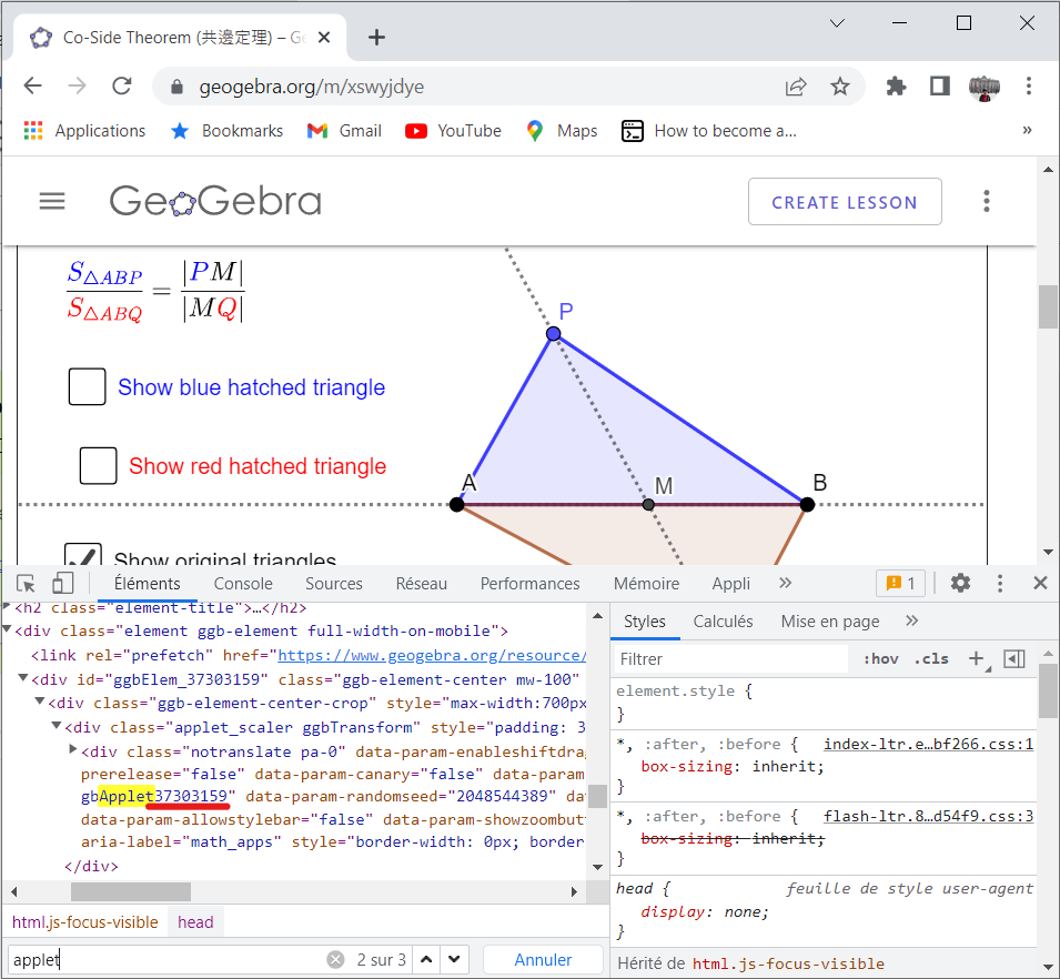
In this example, the desired ID is
37303159. -
Type the first few letters of
ggbAppletin the web developer tools’ console, followed by.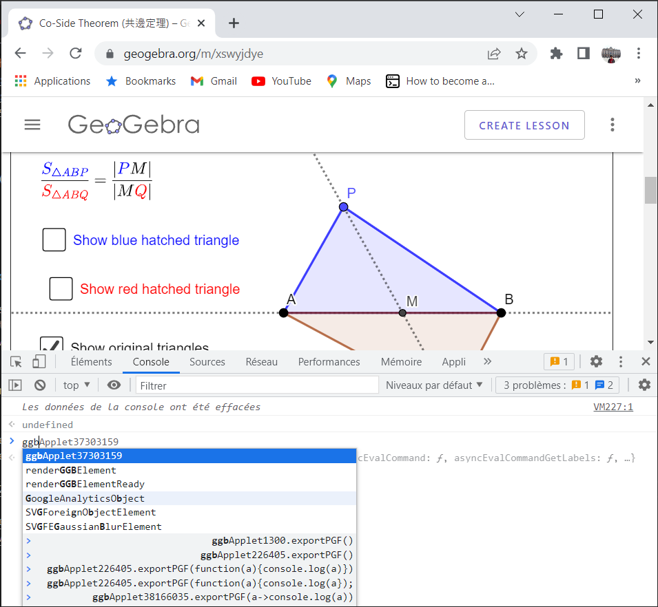
-
Choose the function
exportPGF()with the tab key.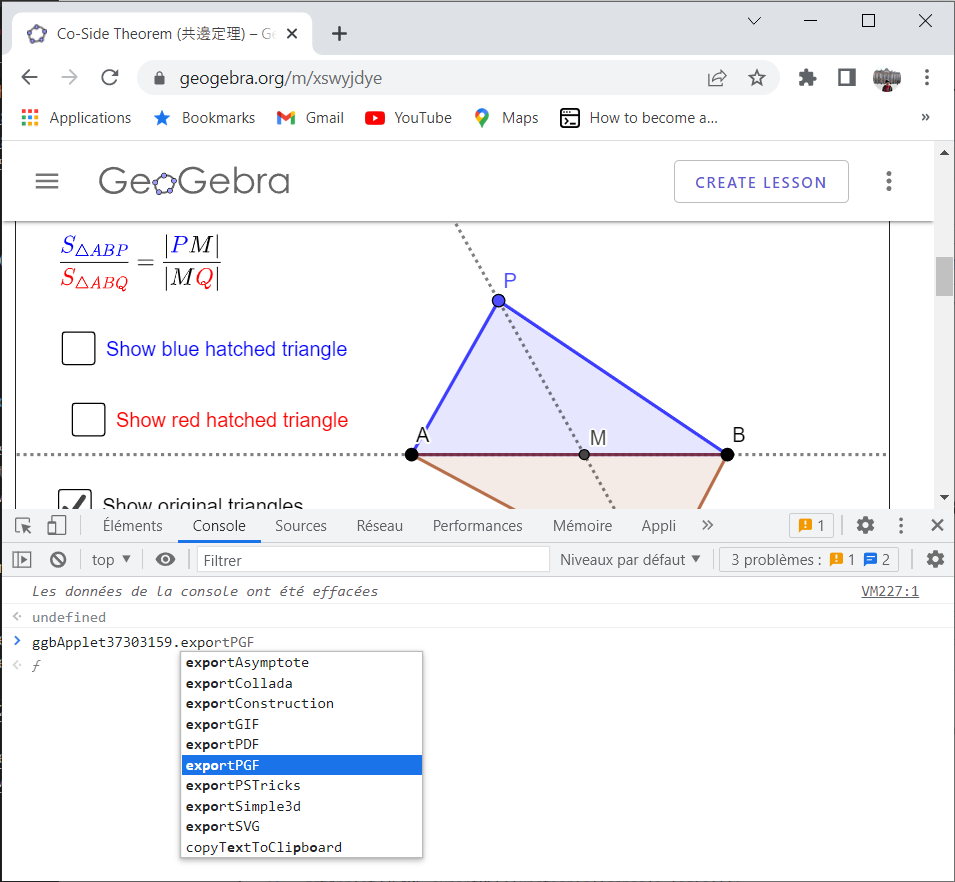
-
Inside the bracket, type
function(a){console.log(a}.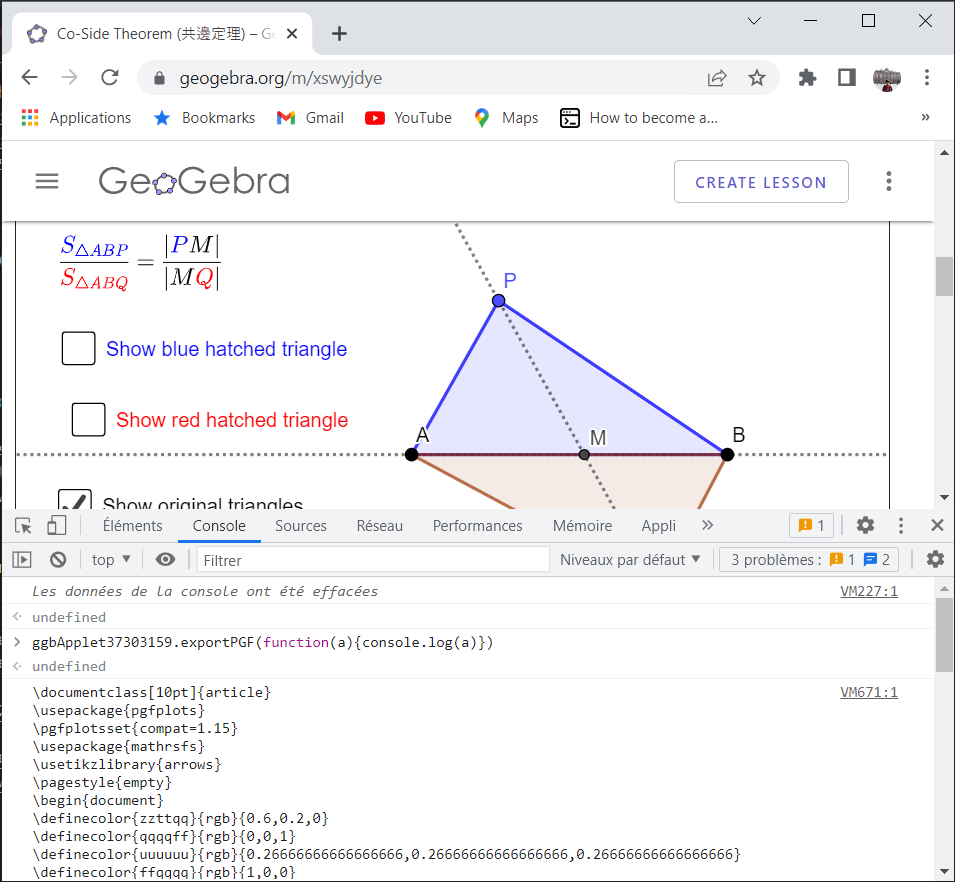
More advanced features
Foreach loops
Example copied from a TeX.SE answer
\documentclass{article}
\usepackage{tikz}
\begin{document}
\begin{tikzpicture}
\foreach \pointA/\pointB in {{(1,0)}/{(2,2)},{(3,4)}/{(2,1)}}{
  \draw \pointA -- \pointB;
}
\end{tikzpicture}
\end{document}
After some testing, I found that the following code works.
\documentclass{article}
\usepackage{tikz}
\begin{document}
\begin{tikzpicture}
\foreach \pointA/\pointB in {
  {(1,0)}/{(2,2)},
  {(3,4)}/{(2,1)}%
} {
  \draw \pointA -- \pointB;
}
\end{tikzpicture}
\end{document}
That’s great especially when there’re
- many loop variables
- many list entries
TikZ’s docs about the auto-loaded PGFFor package provides seperate examples for these keys:
evaluate=<variable>- with an example for
as <macro>to store the evaluation result - without an example for
using <expression>, which should contain at least one reference to<variable>
- with an example for
remember=<variable> as <macro> (initially <value>)seemed too advanced and delicate for me in the past. After struggling with\tikzmath{…}primitive\for{…};loops while often getting compilation errors due to-
omission of final
; -
omission of surrounding
{};in the TikZ command{\draw …;};inside a\forloop -
problem with dynamic evaluation of TikZ
(node\varA name\varB)inside\forloop. I can’t figure out how\expandafterworks inside a\forloop inside\tikzmath{…}.With some experience in array’s reduction/aggregation operation in some programming language (C#, Java, JavaScript), I start appreciating
\foreach \var [
  evaluate=\lastVar as \curVar using <funct(\lastVar)>,
  remember=\curVar as \lastVar initially \valZero
] in \list {…}
like
const valZero = ?;
let list = [?, …, ?];
let curVar = _;  // another variable
let lastVar = valZero;
for (let i = 0; i < list.length; i++) {
  curVar = funct(lastVar);

  // expressions using lastVar and/or curVar and/or list

  lastVar = curVar;
}
In practice, while writing in usual programming languages, we have to take care of each variable’s type and/or scope, slowing down our development. The above usage of
rememberandevaluatewith every optional statement together, which is NOT present in the official docs, can condense code. It has a ‘X’ pattern between\curVarand\lastVar.
-
Here’s a simple template for fractals.
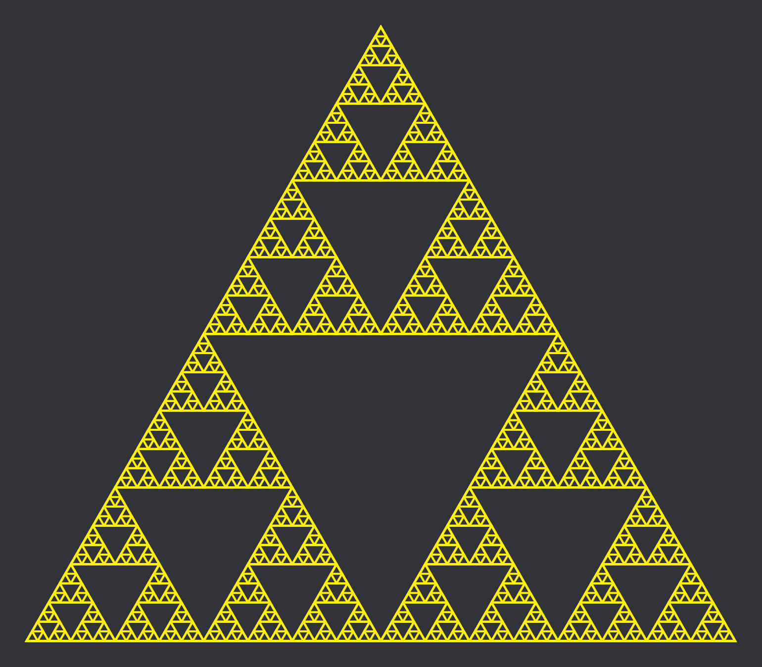
\begin{tikzpicture}
  \path (0,0) coordinate (R0P1);
  \pgfmathsetmacro\myN{7}
  \foreach \ring [
    remember=\ring as \lastRing (initially 0),
    evaluate=\lastNumPoints as \numPoints using int(3*\lastNumPoints),
    remember=\numPoints as \lastNumPoints (initially 1),
    evaluate=\lastBranchLen as \branchLen using \lastBranchLen/2,
    remember=\branchLen as \lastBranchLen (initially 3),
  ] in {1,...,\myN} {
    \foreach \parent in {1,...,\lastNumPoints} {
      \foreach \branch [evaluate=\branch as \sonIdx using int(3*(\parent-1)+\branch+1)] in {0,1,2} {
        \path (R\lastRing P\parent) -- ++({120*\branch+90}:\branchLen) coordinate (R\ring P\sonIdx);
      }
      \draw[yellow] ($(R\lastRing P\parent)+(90:2*\branchLen)$)
        -- ($(R\lastRing P\parent)+(210:2*\branchLen)$)
        -- ($(R\lastRing P\parent)+(330:2*\branchLen)$)
        -- cycle;
    }
  }
\end{tikzpicture}
From each “parent” in the previous “ring” $R_{n-1}P_k$, I declared three new
coordinates $R_nP_{3(k-1)+j}$, where $j \in \lbrace 1, 2, 3 \rbrace$, so that
these new coordinates form an equilateral traingle △ with the parent as its
center, with half of the previous branch length. Using this logic and TikZ’s
pic command, it’s easy to draw fractals of any pattern.

\tikzset{
  heart/.pic={
    \fill[red!40] (0,0) .. controls (0,0.75) and (-1.5,1.00) .. (-1.5,2) arc (180:0:0.75) -- cycle;
    \fill[red!40] (0,0) .. controls (0,0.75) and (1.5,1.00) .. (1.5,2) arc (0:180:0.75) -- cycle;
  }
}
\begin{tikzpicture}
  \path (0,0) coordinate (R0P1);
  \pgfmathsetmacro\myN{5}
  \foreach \ring [
    remember=\ring as \lastRing (initially 0),
    evaluate=\lastNumPoints as \numPoints using int(3*\lastNumPoints),
    remember=\numPoints as \lastNumPoints (initially 1),
    evaluate=\lastBranchLen as \branchLen using \lastBranchLen/2,
    remember=\branchLen as \lastBranchLen (initially 1),
  ] in {1,...,\myN} {
    \foreach \parent in {1,...,\lastNumPoints} {
      \foreach \branch [evaluate=\branch as \sonIdx using int(3*(\parent-1)+\branch+1)] in {0,1,2} {
        \path (R\lastRing P\parent) -- ++({120*\branch+90}:\branchLen) coordinate (R\ring P\sonIdx);
      }
      \pic[scale=0.33*\branchLen] at ([shift={(0,-0.45*\branchLen)}] R\lastRing P\parent) {heart};
    }
  }
\end{tikzpicture}
TikZ math library
Variables
\tikzmath {
  int \f;
  \f = 20;
  print {$f = \f$};
  print \newline;
}
integer: longerintrealcomplex
for-loops (NO while-loops)
“Double quotes” for “text strings”.
\tikzmath{
  for \s in {"a","b","c"} { print {\s}; };
}
Output (in text mode)
a b c
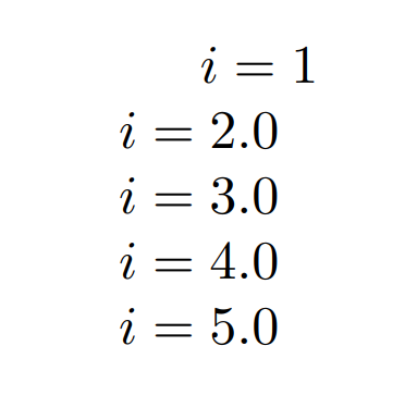
... for ranges.
% documentclass{standalone} won't give new lines, need "article"
\tikzmath{
  for \i in {1,...,5} { print {$i = \i$}; print \newline; };
}
Output
- first line has
\parindent - other lines have
.0
Functions
TikZ’s official site has an example. Instead of copy & pasting, I’ve using my own one, drafted by ChatGPT. This following function won’t work.
\tikzmath{
  int \mynum, \mybase, \highestPow;
  \mynum = 10;
  \mybase = 2;
  function highestPow(\n, \b) {
    if \n == 0 then {return 0;};
    int \d, \tempnum;
    \d = 0;
    \tempnum = \n;
    for \i in {1,...,\tempnum} {
      int \r;
      \r = mod(\tempnum,\b);
      if \r > 0 then {return \d;};
      print {$n = \tempnum$, $d = \d$, $r = \r$};
      print \newline;
      \d = \d + 1;
      \tempnum = \tempnum / \b;
    };
    return \d;
  };
  \highestPow = highestPow(\mynum, \mybase);
  print {The highest power of \mybase{} that divides \mynum{} is \highestPow};
}
returninsideforloop insidefunctionwon’t stopforloop from running.- I can’t do declaration and assignment at the same time.
- I can’t
break;aforloop. - Each
for,if,function, etc, statement ends with a semicolon;. - A TeX.SE user suggested replacing
if [cond] then { "break;" };withif ![cond] then { %TODO }.
An approximation to Cantor set using closed intervals

Commands used
latex temp.tex
dvisvgm -R -d 2 -T "S 2" --font-format=woff temp.dvi -o 240903-cantor-set.svg
\documentclass[preview, margin=2pt, tikz]{standalone}
\usepackage{tikz}
\usetikzlibrary{math}
\begin{document}
\begin{tikzpicture}[scale=6]
\pgfmathsetmacro\myN{5}  % number of levels (i.e. Cantor)
\pgfmathsetmacro\myRowSep{0.2}  % display (non-math) parameter for row separation
\pgfmathsetmacro\myLblSep{1pt}  % display (non-math) parameter for label separation
\tikzmath{ % auxiliary function to find out highest dividing power
  function highestPow(\n, \b) {
    if \n == 0 then {return 0;};
    int \d, \tempnum;
    \d = 0;
    \tempnum = \n;
    for \i in {1,...,\tempnum} {
      if mod(\tempnum,\b) == 0 then { \d = \d + 1; \tempnum = \tempnum / \b; };
    };
    return \d;
  };
}
\foreach \row in {0,...,\myN} {
  \pgfmathsetmacro\numInt{2^\row}  % number of intervals
  \pgfmathsetmacro\intLen{pow(1/3,\row)}  % interval length
  \pgfmathsetmacro\vpos{-\myRowSep*\row}  % display (non-math) param for vertical position
  \node[left=\myLblSep] at (0, \vpos) {$C_\row$};
  % use 1/3 instead of 3 as base to avoid too large value
  \foreach \col [evaluate=\col as \curStep using {\displacement+\intLen+pow(1/3,\row-highestPow(\col,2))},
      remember=\curStep as \displacement (initially 0)] in {1,...,\numInt} {
    \draw (\displacement, \vpos) -- ++(\intLen, 0);
  }
}
\node[above] at (current bounding box.north) {Cantor set $C = \bigcap_{n = 1}^{\infty} C_n$};
\end{tikzpicture}
\end{document}
A step function approximation to Cantor function

In original TikZ code (copied from Discord a couple of years ago), the axis labels aren’t opposing the arrow tip like above. That’s good when there’s no grid. Unluckily, axis labels on top of gray grid lines don’t look nice. After some experiments, I found that when the axis arrow extension is equal to the grid step, the visual outcome is the best.
Apart from that, I applied some tick markings, and a few tick labels, so that they depict some important lengths of the main character, without overcrowding the axis with too many labels.
On the Discord version, I used \draw[yellow, thick] so that the curve is more
visible. An opacity of 0.5 is applied to let the main character shine.
\documentclass[preview, margin=2pt, tikz]{standalone}
\usepackage{tikz}
\usetikzlibrary{math}
\begin{document}
\begin{tikzpicture}[scale=6]
\pgfmathsetmacro\myN{8}  % number of levels, must be greater than one
\pgfmathsetmacro\myRowSep{0.5^\myN}  % row separation
\pgfmathsetmacro\myLblSep{1pt}  % display (non-math) parameter for label separation
\pgfmathsetmacro\myPadding{.05} % display (non-math) parameter for extra axis length

\draw[help lines, step=0.05cm] (0,0) grid (1,1);
% x-axis
\draw[thick] [->] (-\myPadding,0) -- (1+\myPadding,0) node [right] {$x$};
\foreach \x in {0,0.111,...,1} {
  \draw[xshift=\x cm, opacity=.5] (0pt,-.5pt)--(0pt,.5pt);
};
% y-axis
\draw[thick] [->] (0,-\myPadding) -- (0,1+\myPadding) node [above] {$y$};
\foreach \y in {0,0.0625,...,1} {
  \draw[yshift=\y cm, opacity=.5] (-.5pt,0pt)--(.5pt,0pt);
};
% tick labels
\path (0,0) node[below left] {$O$};
\foreach \x in {1/3, 2/3, 1} {\node[below] at (\x,0) {$\x$};};
\foreach \y in {1/4, 1/2, 3/4, 1} {\node[left] at (0,\y) {$\y$};};

\tikzmath{ % auxiliary function to find out highest dividing power
  function highestPow(\n, \b) {
    if \n == 0 then {return 0;};
    int \d, \tempnum;
    \d = 0;
    \tempnum = \n;
    for \i in {1,...,\tempnum} {
      if mod(\tempnum,\b) == 0 then { \d = \d + 1; \tempnum = \tempnum / \b; };
    };
    return \d;
  };
}
\pgfmathsetmacro\numInt{2^\myN-1}  % number of intervals
\pgfmathsetmacro\intLen{pow(1/3,\myN)}  % interval length
% use 1/3 instead of 3 as base to avoid too large value
\foreach \col [evaluate=\col as \curStep using {\displacement+\intLen+pow(1/3,\myN-highestPow(\col,2))},
    remember=\curStep as \displacement (initially 0)] in {1,...,\numInt} {
  \draw (\displacement+\intLen, \col*\myRowSep) -- ++({pow(1/3,\myN-highestPow(\col,2))}, 0);
};
\node[above] at (current bounding box.north) {Cantor function $c(x)$ with $n = \myN$};
\node[above] at (current bounding box.north) {Step function approximation for};
\end{tikzpicture}
\end{document}
An illustration to a homeomorphism ψ : [0, 1] → [0, 2], ψ := id + c, where c is Cantor function.
This function is used for constructing a Lebesgue measurable set which is NOT Borel.

\documentclass[preview, margin=2pt, tikz]{standalone}
\usepackage{tikz}
\usetikzlibrary{math}
\begin{document}
\begin{tikzpicture}[scale=6]
\pgfmathsetmacro\myN{6}  % number of levels
\pgfmathsetmacro\myRowSep{0.5^\myN}
\pgfmathsetmacro\myLblSep{1pt}  % display parameter for label separation
\pgfmathsetmacro\myPadding{.05} % display parameter for extra axis length

\draw[help lines, step=0.05cm] (0,0) grid (1,2);
% x-axis
\draw[thick,->] (-\myPadding,0) -- (1+\myPadding,0) node [right] {$x$};
\foreach \x in {0,0.111,...,1} {
  \draw[xshift=\x cm] (0pt,-.5pt)--(0pt,.5pt);
};
% y-axis
\draw[thick,->] (0,-\myPadding) -- (0,2+\myPadding) node [above] {$y$};
\foreach \y in {0,0.0625,...,2} {
  \draw[yshift=\y cm] (-.5pt,0pt)--(.5pt,0pt);
};
% tick labels
\path (0,0) node[below left] {$O$};
\foreach \x in {1/3, 2/3, 1} {\node[below] at (\x,0) {$\x$};};
\foreach \y in {1/4, 1/2, 3/4, 1, 5/4, 3/2, 7/4, 2} {\node[left] at (0,\y) {$\y$};};

\tikzmath{ % auxiliary function
  function highestPow(\n, \b) {
    if \n == 0 then {return 0;};
    int \d, \tempnum;
    \d = 0;
    \tempnum = \n;
    for \i in {1,...,\tempnum} {
      if mod(\tempnum,\b) == 0 then { \d = \d + 1; \tempnum = \tempnum / \b; };
    };
    return \d;
  };
}
\pgfmathsetmacro\numInt{2^\myN-1}  % number of intervals
\pgfmathsetmacro\intLen{pow(1/3,\myN)}  % interval length
% avoid too large base
\foreach \col [evaluate=\col as \curStep using {\displacement+\intLen+pow(1/3,\myN-highestPow(\col,2))},
    remember=\curStep as \displacement (initially 0)] in {1,...,\numInt} {
  \draw (\displacement+\intLen, \displacement+\intLen+\col*\myRowSep)
    -- ++({pow(1/3, \myN-highestPow(\col,2))}, {pow(1/3, \myN-highestPow(\col,2))});
};
\node[above, text width=6cm] at (current bounding box.north) {Piecewise linear approximation for homeomorphism $\psi(x) = c(x) + x$ with $n = \myN$};
\end{tikzpicture}
\end{document}